📖 Mathematical Statistics

This module continuously compiles core foundational concepts related to mathematical statistics.

1. Hypothesis Testing and Confusion Matrix

Under the frequentist Neyman-Pearson framework, hypothesis testing is essentially a binary decision-making process based on a sample regarding the true parameter space.

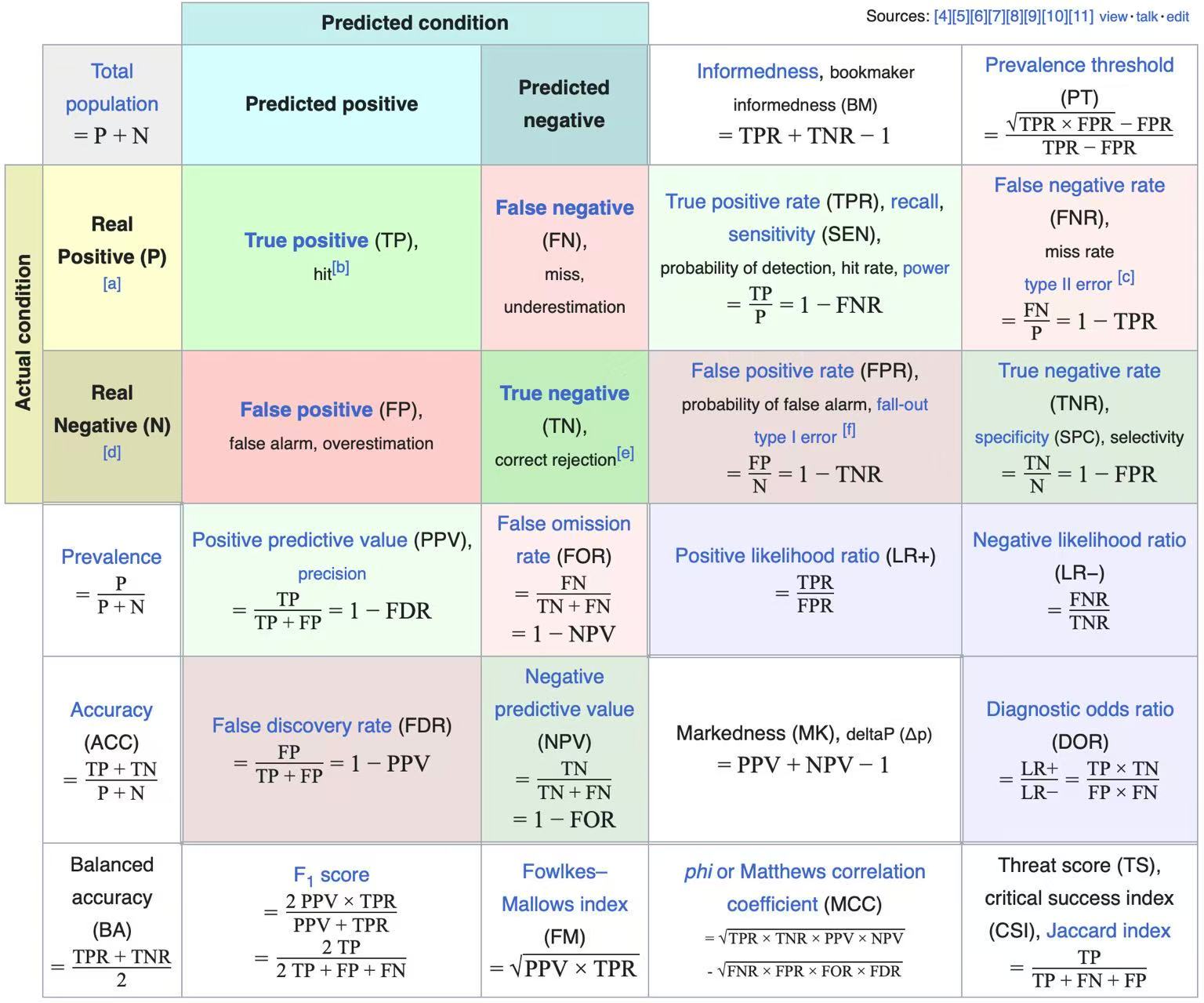
Hypothesis Testing Confusion Matrix

True State \ Model Prediction	Accept \(H_0\) (Do not reject)	Reject \(H_0\) (Reject, Discover)
\(H_0\) is True (Null is True)	✅ Correct Inference (True Negative, \(1-\alpha\))	❌ Type I Error (False Positive, \(\alpha\))
\(H_1\) is True (Alt is True)	❌ Type II Error (False Negative, \(\beta\))	✅ Statistical Power (True Positive, Power: \(1-\beta\))

Core Concepts Quick Reference

Type I Error (False Positive)

Definition: The null hypothesis \(H_0\) is true, but it is incorrectly rejected. Also known as a "false alarm."
Mathematical Expression: \(\alpha = P(\text{Reject } H_0 \mid H_0 \text{ is True}) = \frac{FP}{FP+TN}\)
Alias: The Significance Level of the test. In classical statistics, we usually strictly control \(\alpha\) first (e.g., setting it to \(0.05\)).

Type II Error (False Negative)

Definition: The alternative hypothesis \(H_1\) is true, but we fail to reject \(H_0\). Also known as a "miss."
Mathematical Expression: \(\beta = P(\text{Accept } H_0 \mid H_1 \text{ is True}) = \frac{FN}{TP+FN}\)

Statistical Power

Definition: The probability of correctly rejecting \(H_0\) when the alternative hypothesis \(H_1\) is true. It represents the ability of the test to detect a true effect.
Mathematical Expression: \(\text{Power} = 1 - \beta = P(\text{Reject } H_0 \mid H_1 \text{ is True}) = \frac{TP}{TP+FN}\)
Intuition: Given a fixed \(\alpha\), we aim to find testing methods that maximize Power (i.e., the Uniformly Most Powerful test, or UMP test).

p-value

Definition: The probability of observing the current sample statistic (or one more extreme) given that the null hypothesis \(H_0\) is true.
Pitfall: A p-value is absolutely not the "probability that the null hypothesis is true" (i.e., \(p \ne P(H_0 \mid \text{Data})\)). It reflects the degree of inconsistency between the data and the null hypothesis. The smaller the p-value, the stronger the evidence to reject \(H_0\).

Modern Frontiers: Multiple Testing and FDR Control

In modern high-dimensional statistics, we often need to perform thousands of tests simultaneously. In such cases, traditional \(\alpha\) control fails completely.

The Multiple Testing Problem

Suppose we independently test \(m\) completely ineffective factors (i.e., \(m\) null hypotheses \(H_0\) all hold), with a single-test significance level of \(\alpha = 0.05\).

Then the probability of making at least one Type I error (Family-Wise Error Rate, FWER) is:

\[ \text{FWER} = P(V \ge 1) = 1 - (1 - \alpha)^m \]

When \(m = 100\), \(\text{FWER} \approx 0.994\). This means that if you test enough factors, you are almost guaranteed to find seemingly significant "spurious signals." This necessitates the concept of FDR.

FDR (False Discovery Rate)

Proposed by Benjamini and Hochberg in 1995, this is a core concept in high-dimensional inference.

Definition: The expected value of the proportion of incorrect rejections (Type I errors \(V\)) among all rejected null hypotheses (total discoveries \(R\)).

\[ \text{FDR} = E\left[ \frac{V}{\max(R, 1)} \right] = \frac{FP}{TP+FP} \]

BH Procedure (Benjamini-Hochberg Procedure):
1. Sort the p-values of the \(m\) hypotheses in ascending order: \(p_{(1)} \le p_{(2)} \le \dots \le p_{(m)}\).
2. Find the largest integer \(k\) such that \(p_{(k)} \le \frac{k}{m} \alpha\).
3. Reject the first \(k\) null hypotheses (i.e., \(H_{(1)}, \dots, H_{(k)}\)).
4. Theorem: Under the assumption of independence (or positive dependence), this procedure strictly controls the FDR \(\le \alpha\).

Hyphothesis Testing Table

2. Order Statistics

Let \(X_1, X_2, \dots, X_n\) be i.i.d. samples from a population with distribution \(F(x)\) and density \(f(x)\). Arranging them in ascending order \(X_{(1)} \le X_{(2)} \le \dots \le X_{(n)}\), we call \(X_{(k)}\) the \(k\)-th order statistic.

Core Distribution Formulas

PDF of a Single Order Statistic (\(X_{(k)}\))

The probability density function of the \(k\)-th order statistic \(X_{(k)}\) is:

\[f_{(k)}(x) = \frac{n!}{(k-1)!(n-k)!} [F(x)]^{k-1} [1-F(x)]^{n-k} f(x)\]

Heuristic Derivation: Multinomial Perspective

Consider a tiny interval \([x, x+dx]\) around \(x\). The event that \(X_{(k)}\) falls in this interval is equivalent to:

Exactly 1 sample falls in \([x, x+dx]\), with probability approximately \(f(x)dx\).
Exactly \(k-1\) samples fall in \((-\infty, x)\), with probability \([F(x)]^{k-1}\).
The remaining \(n-k\) samples fall in \((x+dx, \infty)\), with probability \([1-F(x)]^{n-k}\).

Using multinomial coefficients for permutations, the total number of ways is \(\frac{n!}{(k-1)! \cdot 1! \cdot (n-k)!}\). Multiplying these terms and canceling \(dx\) yields the PDF formula above.

Distributions of Extrema (Special Cases)

Most commonly used in reliability engineering and extreme value theory:

Minimum \(X_{(1)}\): \(f_{(1)}(x) = n[1-F(x)]^{n-1} f(x)\)
Maximum \(X_{(n)}\): \(f_{(n)}(x) = n[F(x)]^{n-1} f(x)\)

Important Properties and Conclusions

Joint Distribution

The joint probability density function of all order statistics is:

\[f_{(1), \dots, (n)}(x_1, \dots, x_n) = \begin{cases} n! \prod_{i=1}^n f(x_i) & x_1 < x_2 < \dots < x_n \\ 0 & \text{otherwise} \end{cases}\]

(Intuition: This is equivalent to "stacking" the joint density of the original sample \(n!\) times over the ordered space).

The Uniform Connection

Let \(U_{(k)}\) be the \(k\)-th order statistic from a \(U(0, 1)\) distribution, then:

Beta Distribution: \(U_{(k)} \sim \text{Beta}(k, n-k+1)\).
Expectation and Variance: \(E[U_{(k)}] = \frac{k}{n+1}\). This is crucial for understanding Quantile estimation.
Probability Integral Transform: For any continuous distribution \(F(x)\), \(F(X_{(k)}) \overset{d}{=} U_{(k)}\).

Joint Distributions of Multiple Order Statistics

In non-parametric inference and survival analysis, we often study the relationship between specific ranked observations.

Joint Density of Two Order Statistics (\(i < j\))

Let \(1 \le i < j \le n\). The joint PDF of \(X_{(i)}\) and \(X_{(j)}\) is:

\[f_{(i),(j)}(u, v) = \frac{n!}{(i-1)!(j-i-1)!(n-j)!} [F(u)]^{i-1} f(u) [F(v)-F(u)]^{j-i-1} f(v) [1-F(v)]^{n-j}\]

where \(u < v\), and 0 otherwise.

Multinomial Heuristic Derivation

Imagine \(n\) sample points partitioned into 5 distinct intervals:

\((-\infty, u)\): Contains \(i-1\) points, with probability \(F(u)\).
\([u, u+du]\): Contains 1 point (\(X_{(i)}\)), with probability \(f(u)du\).
\((u+du, v)\): Contains \(j-i-1\) points, with probability \(F(v)-F(u)\).
\([v, v+dv]\): Contains 1 point (\(X_{(j)}\)), with probability \(f(v)dv\).
\((v+dv, \infty)\): Contains \(n-j\) points, with probability \(1-F(v)\).

Based on the multinomial formula, the number of permutations is \(\frac{n!}{(i-1)! 1! (j-i-1)! 1! (n-j)!}\). Multiplying the probabilities of each interval by their respective powers and canceling \(du, dv\) yields the formula. This logic extends to the joint distribution of any \(k\) order statistics.

Range and Median

Distribution of the Sample Range

The range is defined as \(R = X_{(n)} - X_{(1)}\). For a \(U(0, 1)\) distribution, the PDF of the range is:

\[f_R(r) = n(n-1)r^{n-2}(1-r), \quad 0 < r < 1\]

(The derivation requires writing the joint distribution of \(X_{(1)}\) and \(X_{(n)}\) first, then performing a bivariate transformation).

Core Derivation Steps: From Joint to Marginal Distribution

Step 1: Write the joint distribution of \(X_{(1)}\) and \(X_{(n)}\) Setting \(i=1, j=n\) in the general joint formula:

\[f_{(1),(n)}(u, v) = n(n-1) [F(v)-F(u)]^{n-2} f(u) f(v), \quad u < v\]

Step 2: Bivariate Transformation Introduce the range \(R\) and an auxiliary variable \(V\) (usually the minimum):

\[\begin{cases} R = X_{(n)} - X_{(1)} \\ V = X_{(1)} \end{cases} \implies \begin{cases} X_{(1)} = V \\ X_{(n)} = R + V \end{cases}\]

The Jacobian determinant is: \(|J| = \left| \frac{\partial(u, v)}{\partial(r, v)} \right| = \det \begin{pmatrix} 0 & 1 \\ 1 & 1 \end{pmatrix} = |-1| = 1\).

Step 3: Find the joint density of \(R\) and \(V\)

\[f_{R,V}(r, v) = f_{(1),(n)}(v, r+v) \cdot |J| = n(n-1) [F(r+v)-F(v)]^{n-2} f(v) f(r+v)\]

Step 4: Integrate over \(V\) to find the marginal density of \(R\)

\[f_R(r) = \int_{-\infty}^{\infty} n(n-1) [F(r+v)-F(v)]^{n-2} f(v) f(r+v) dv, \quad r > 0\]

Asymptotic Property

As \(n \to \infty\):

Sample Median: Under certain conditions, it converges to a normal distribution (a variant of the Central Limit Theorem).
Sample Extrema: Converge to one of three extreme value distributions (Gumbel, Fréchet, or Weibull), which is the core of Extreme Value Theory (EVT).